VLOOKUP Function in Excel
VLOOKUP is a powerful tool in Microsoft Excel that can instantly find (Lookup) items in a Data Set and bring their corresponding values from the same or another spreadsheet. For example, take the case of a Sales Data containing Names of items sold in one column and their corresponding selling Prices in another column. In this case, the VLOOKUP Function can be used to list the Price of Items by looking up Item Names in the ‘Names’ Column and their corresponding Prices located in another column. To understand this better, let us go ahead and take a look at the Syntax and the steps to use VLOOKUP Function in Excel.
1. Syntax of VLOOKUP Formula
Microsoft Excel automatically provides you with the syntax for VLOOKUP Function as soon as you start entering =VLOOKUP in any cell of an Excel Spreadsheet. Hence, there is really no need to remember the Syntax of VLOOKUP Function. However, you do need to understand the Syntax, in order to clearly understand this function. The VLOOKUP function has the following Syntax: =VLOOKUP (Lookup_value , Table_array, Col_index_num , [range_lookup] ) Lookup_Value: This is the item that you want to lookup. Table_Array: This is where the data to lookup is located. Col_Index_Num: Column Number from which the lookup value should be returned. [Range_Lookup]: This can be either True or False. If the specified parameter is True, VLOOKUP searches for the approximate or nearest match. If the specified parameter is False, VLOOKUP searches for the exact match.
2. How to Use VLOOKUP Function in Excel
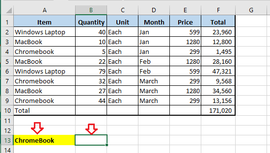
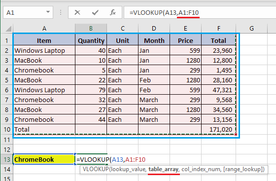
The Sales Data as provided below has item Names in Column A and corresponding Prices of these items in Column E. The task in this example is to use the VLOOKUP Function to lookup (Chromebook) and bring up the price of Chromebook in Cell B13.
Start by typing the Name of item that you want to lookup in Cell A13 – In our case, the item that we want to lookup is Chromebook.
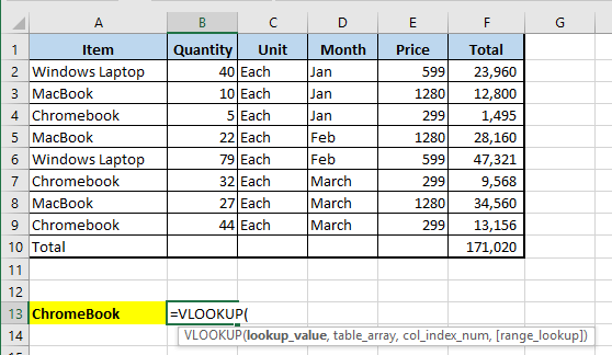
Next, start typing =VLOOKUP in Cell B13 and Excel will automatically provide you with the Syntax to follow.
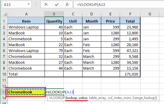
Going by the Syntax, select Cell E3 as the Lookup_value – This is where you typed the Name of item that you want to Lookup (Chromebook).
Next, select Cells A1:F10 as the Table_array – This is where the data that you want to scan is located.
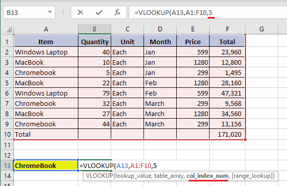
The next part is Column_Index_Num – Type 5 to indicate that the price of item (Chromebook) that you want to lookup is located in the 5th column from left.
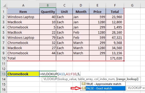
The last part is [Range_Lookup]: As explained above, simply pick False to indicate that you want to find the exact match for the price of Chromebook.
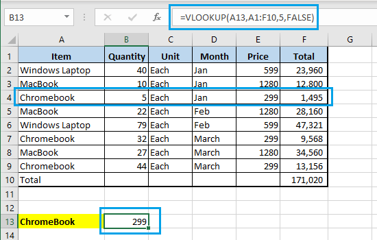
Close the bracket and hit the Enter Key on the keyboard of your computer.
Once you hit the Enter Key, VLOOKUP function will lookup (Chromebook) in Column A and bring up the price of Chromebook from Column E. While the above example is a very simple one, you can trust the VLOOKUP function to work flawlessly, when you are dealing with large amounts of data.
How to Use Concatenate Function in Excel How to Add Prefix or Suffix in Excel